SDForest

Here, we show the functionality of an SDForest and how you can use it to screen for causal parents of a continuous response in a large set of observed covariates, even in the presence of hidden confounding. We also provide methods to asses the functional partial dependence of the response on the causal parents.

We show the functionalities with simulated data from a confounded model with one true causal parents of $Y$, see simulate_data_nonlinear().

library(SDModels)
set.seed(42)
# simulation of confounded data
q <- 2    # dimension of confounding
p <- 350  # number of overved covariates
n <- 400  # number of obervations
m <- 1    # number of causal parents in covariates

sim_data <- simulate_data_nonlinear(q = q, p = p, n = n, m = m)
X <- sim_data$X
Y <- sim_data$Y
train_data <- data.frame(X, Y)

# causal parents of y
f <- apply(X, 1, function(x) f_four(x, sim_data$beta, sim_data$j))

# functional dependence on causal parents
plot(x = X[, sim_data$j], f, xlab = paste0('X_', sim_data$j))

# observed dependence on causal parents
plot(x = X[, sim_data$j], Y, xlab = paste0('X_', sim_data$j))

We first estimate the random forest using the spectral objective:

$$\hat{f} = \text{argmin}_{f' \in \mathcal{F}} \frac{||Q(\mathbf{Y} - f'(\mathbf{X}))||_2^2}{n}$$ where $Q$ is a spectral transformation. (Ćevid, Bühlmann, and Meinshausen 2020)

fit <- SDForest(Y ~ ., train_data)
fit
#> SDForest result
#> 
#> Number of trees:  100 
#> Number of covariates:  350 
#> OOB loss:  1.19 
#> OOB spectral loss:  0.02

Causal parents

Given the estimated causal function, the first question we might want to answer is which of the covariates are the causal parents of the response. If we intervene on the causal parents, we expect the response to change. For that, we can estimate the functional dependency of $Y$ on $X$, $\widehat{f(X)}$ and examine which covariates are important in this function. We can directly compare the importance pattern of the deconfounded estimator to the classical random forest estimated by ranger. This comparison to the plain counterpart always gives a feeling of the strength of confounding. If no confounding exists, SDForest() and ranger::ranger() should result in similar models.

In the graph below, we see the variable importance varImp() of the deconfounded random forest against the plain random forest. The scale has no meaning, but we see how the true causal parents in red is getting a clear higher variable importance for the SDForest. The plain random forest cannot distinguish between spurious correlation and true causation.

# comparison to classical random forest
fit_ranger <- ranger::ranger(Y ~ ., train_data, importance = 'impurity')

# comparison of variable importance
imp_ranger <- fit_ranger$variable.importance
imp_sdf <- fit$var_importance
imp_col <- rep('black', length(imp_ranger))
imp_col[sim_data$j] <- 'red'

plot(imp_ranger, imp_sdf, col = imp_col, pch = 20,
     xlab = 'ranger', ylab = 'SDForest', 
     main = 'Variable Importance')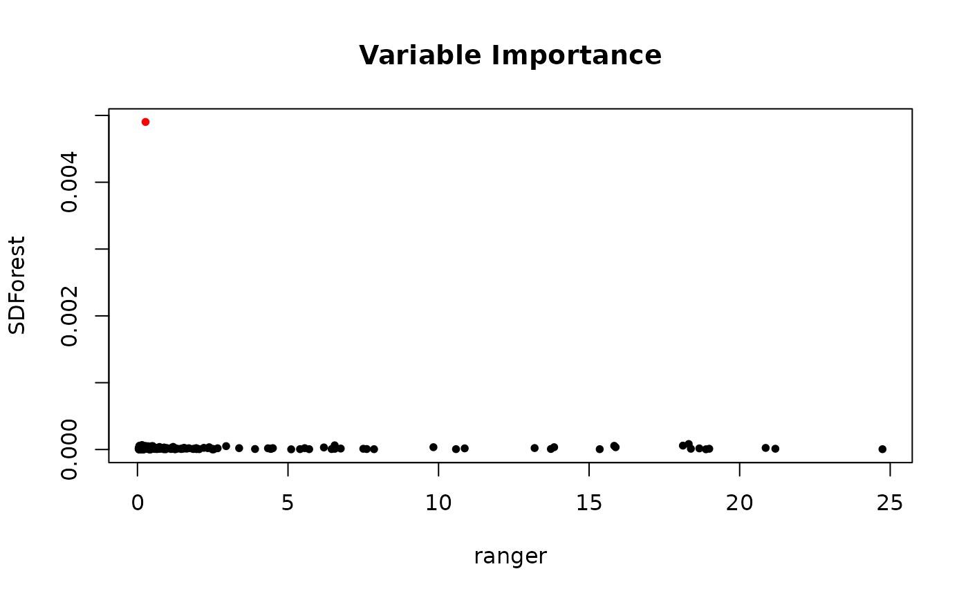

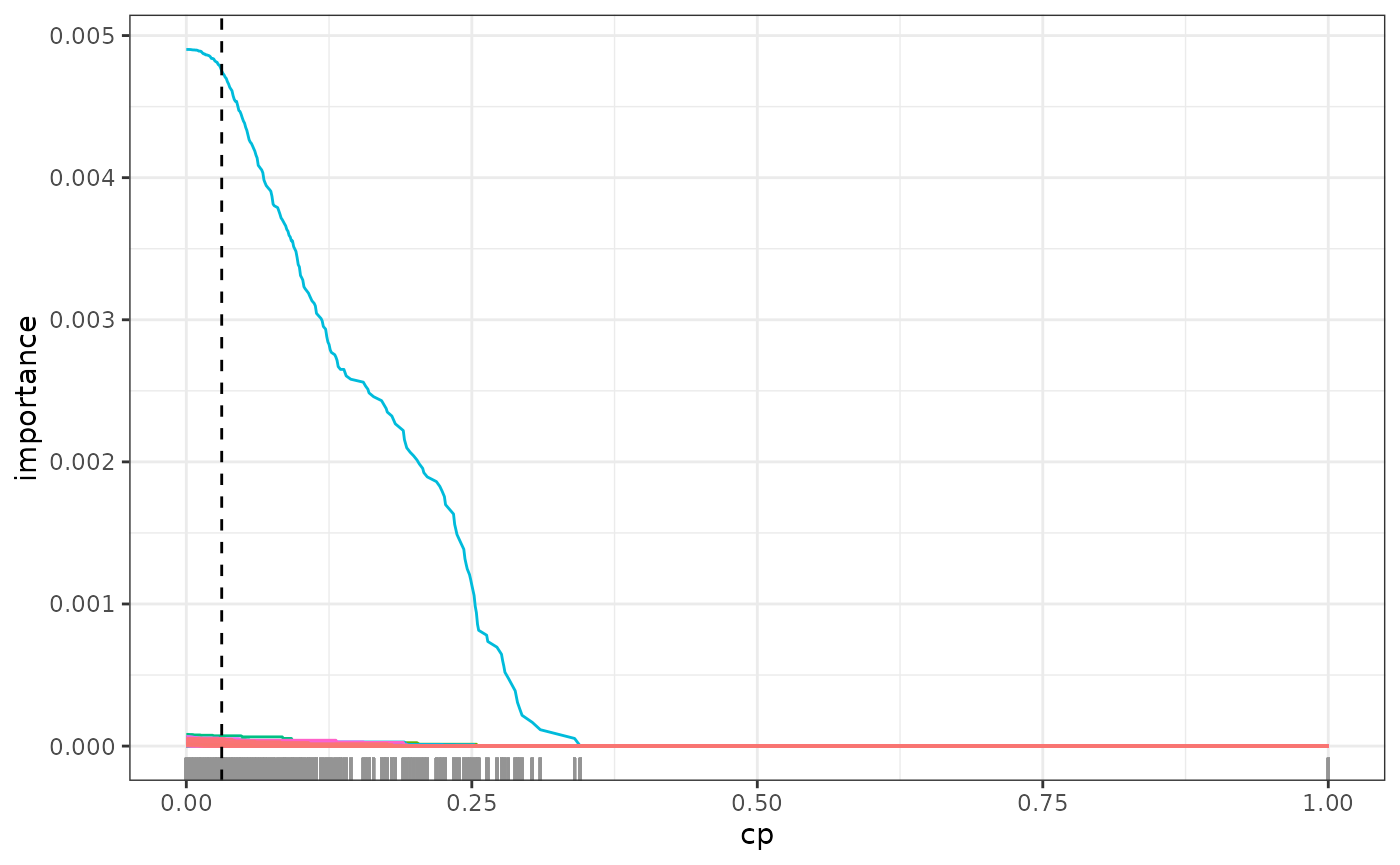
Before, we looked at the variable importance of the non-regularized SDForest. We have two more techniques to better understand which variables might be causally important. The first is the regularization path regPath(), where we plot the variable importance against varying regularization, i.e. different cp values. The option plotly = TRUE lets us visualize these paths interactively to better understand which covariates seem to have robust importance in the model.

# check regularization path of variable importance
path <- regPath(fit)
plot(path)

# select 20 most important covariates for further exploration
most_imp <- fit$var_importance > sort(fit$var_importance, decreasing = TRUE)[20]
plot(path, plotly = TRUE, most_imp)

The second method follows the stability selection approach (Meinshausen and Bühlmann 2010). Here, we visualize the proportion of trees in the forest that use each covariate for splits in the model. As we regularize more, only the truly causal important variables will still be used by most trees.

# detection of causal parent using stability selection
stablePath <- stabilitySelection(fit)
#plot(stablePath, plotly = TRUE)
plot(stablePath)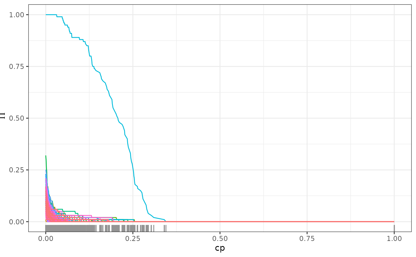

Causal dependence

After finding the causal parent of the response, one might be interested in the partial functional dependence of $Y$ on the causal parents. If we want to intervene in a system, we need to not only know where to intervene but also how to intervene in order to get the desired response. For that, we first prune the forest to remove any residual spurious correlation and get optimal predictive power. For that, regPath() also contains the out-of-bag prediction errors for different regularizations. plotOOB() visualizes both the mean squared error (oob.MSE) and the spectral loss (oob.SDE) that we minimize. The minimal out-of-bag error lets us choose the optimal cp value to prune the forest.

# out of bag error for different regularization
plotOOB(path)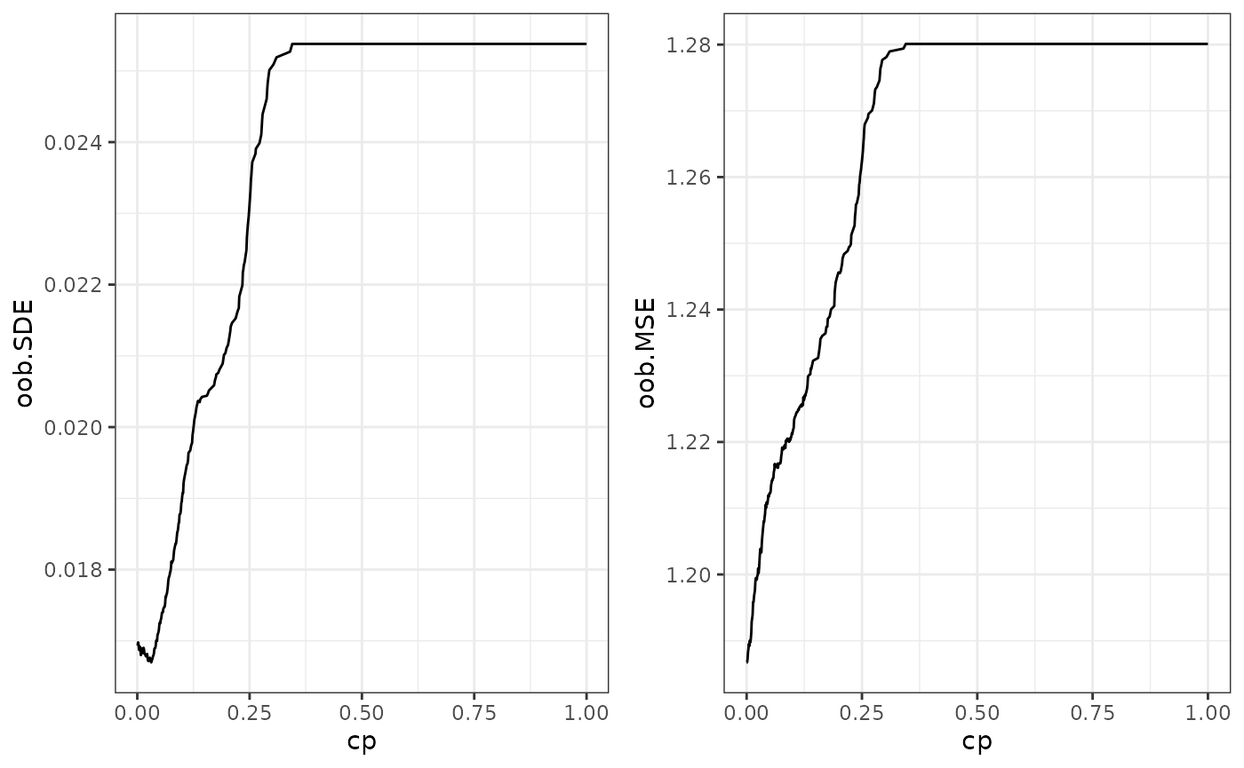

path$cp_min
#> [1] 0.031

# pruning of forest according to optimal out-of-bag performance
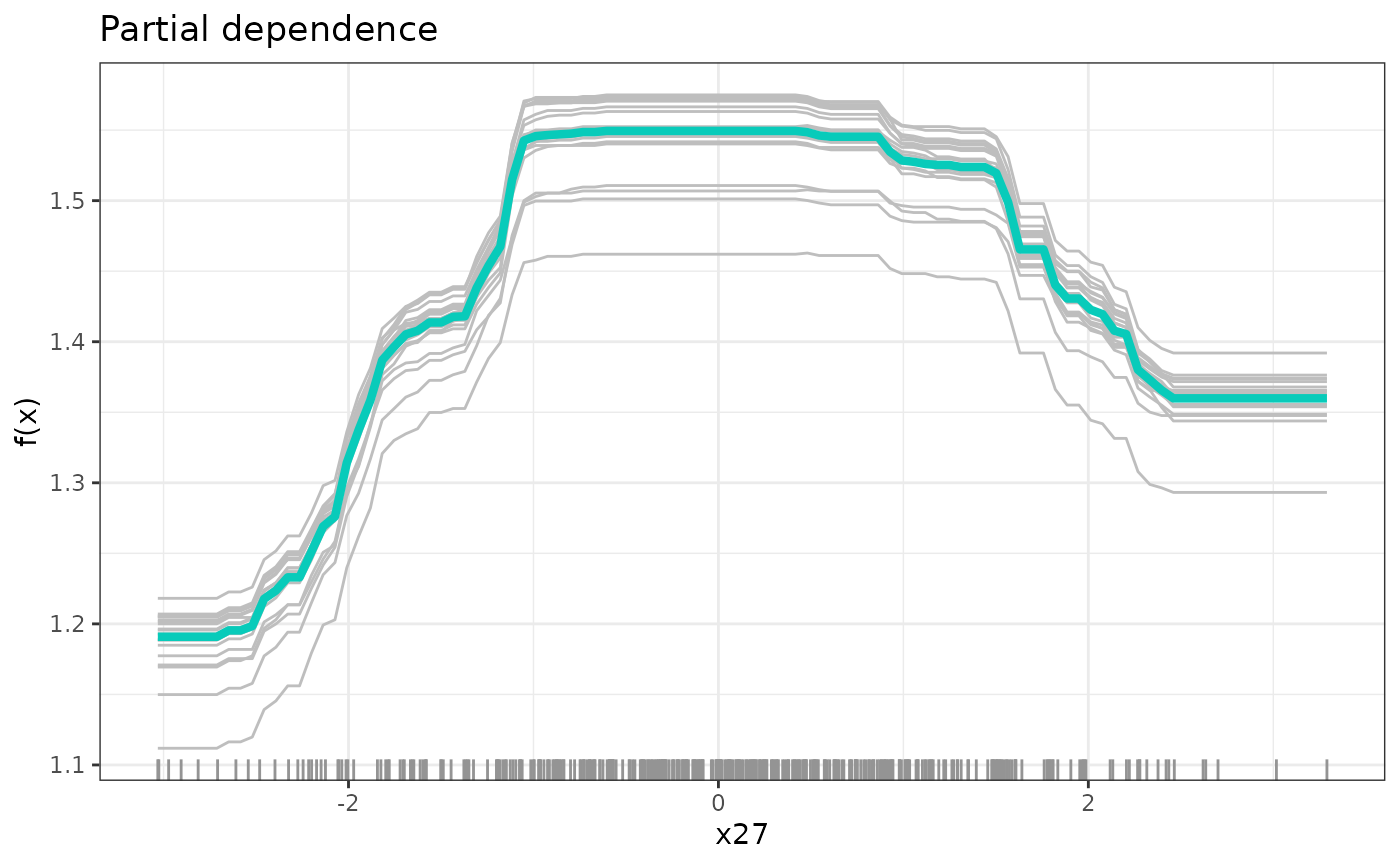
fit <- prune(fit, cp = path$cp_min)

Now, to distil the partial functional dependence of the response on the causal parents, we use partial dependence plots in partDependence() (Friedman 2001). For that, we vary the value of one covariate while fixing the others to the ones that we actually observe in the data. As representative partial conditional dependence, we plot the mean over these individual response curves in addition to a few sample individuals.

# partial functional dependence of y on the first causal parent
dep <- partDependence(fit, sim_data$j)
plot(dep)

Ćevid, Domagoj, Peter Bühlmann, and Nicolai Meinshausen. 2020. “Spectral Deconfounding via Perturbed Sparse Linear Models.” J. Mach. Learn. Res. 21 (1). http://jmlr.org/papers/v21/19-545.html.

Friedman, Jerome H. 2001. “Greedy Function Approximation: A Gradient Boosting Machine.” The Annals of Statistics 29 (5): 1189–1232. http://www.jstor.org/stable/2699986.

Meinshausen, Nicolai, and Peter Bühlmann. 2010. “Stability Selection.” Journal of the Royal Statistical Society Series B: Statistical Methodology 72 (4): 417–73. https://doi.org/10.1111/j.1467-9868.2010.00740.x.