SDAM

In the following, we show the functionality of SDAM and show how it can be used to fit a high-dimensional additive model in the presence of hidden confounding and how to analyze the fitted model. SDAM is an implementation of the algorithm described in (Scheidegger, Guo, and Bühlmann 2025), where also a systematic simulation study can be found.

We first simulate some data that is confounded. We assume the data generating process $$Y= f(X) + \delta^T H + \nu, \quad X = \Gamma^TH + E,$$ where the function $f$ is additive in the first 4 covariates.

set.seed(99)

# function f is additive in the first 4 covariates
f1 <- function(x){-sin(2*x)}
f2 <- function(x){2-2*tanh(x+0.5)}
f3 <- function(x){x}
f4 <- function(x){4/(exp(x)+exp(-x))}
f <- function(X){f1(X[,1])+f2(X[,2])+f3(X[,3])+f4(X[,4])}

n <- 300
p <- 200
q <- 5

Gamma <- matrix(runif(q*p, min = -1, max = 1), nrow=q)
delta <- runif(q, min = 0, max = 2)
H <- matrix(rnorm(n*q), nrow = n)
E <- matrix(rnorm(n*p), nrow = n)
nu <- 0.5*rnorm(n)
X <- H %*% Gamma + E
Y <- f(X) + H %*% delta + nu

The goal is to estimate the function $f$. We fit both a standard additive model and a deconfounded additive model using the trim transformation.

library(SDModels)
fit_standard <- SDAM(x = X, y = Y, Q_type = "no_deconfounding")
#> [1] "Initial cross-validation"
#> [1] "Second stage cross-validation"
fit_trim <- SDAM(x = X, y = Y, Q_type = "trim")
#> [1] "Initial cross-validation"
#> [1] "Second stage cross-validation"

For both models, we compare the predicted values to the true function $f$ by calculating the mean squared error on the training data.

pred_standard <- predict(fit_standard, newdata = data.frame(X))
pred_trim <- predict(fit_trim, newdata = data.frame(X))

(MSE_standard <- mean((f(X) - pred_standard)^2))
#> [1] 10.00365
(MSE_trim <- mean((f(X) - pred_trim)^2))
#> [1] 0.73134

We see that the mean squared error when using the deconfounding is smaller than using no spectral transformation. Let us have a look at the variable importance.

plot(varImp(fit_standard), main = "Standard Additive Model", xlab = "j", ylab = "variable importance")

plot(varImp(fit_trim), main = "Deconfounded Additive Model", xlab = "j", ylab = "variable importance")

We see that both methods attribute the largest effects to variables in the active set. However, when using deconfounding, there is much less signal that is captured from other covariates, whereas a plain additive model also attributes significant influence to the non-active covariates and also completely ignores the effect of $X_1$. We can get the size of the active set by using the function and see that when using deconfounding, we get a smaller set of active variables.

print(fit_standard)
#> SDAM result
#> 
#> Number of covariates:  200 
#> Number of active covariates:  85
print(fit_trim)
#> SDAM result
#> 
#> Number of covariates:  200 
#> Number of active covariates:  20

Let us finally have a look at the individual component functions $f_j$. They can be displayed using the function. We display the individual component functions $f_j$ for $j\in \{1,2,3,4\}$ (true active set).

xx <- seq(-4, 4, 0.05)
XX <- data.frame(matrix(rep(seq(-4, 4, 0.05), p), ncol = p))

for(j in 1:4){
  fj <- get(paste("f", j, sep = ""))
  predj_standard <- predict_individual_fj(fit_standard, j, XX)
  predj_trim <- predict_individual_fj(fit_trim, j, XX)
  plot(xx, fj(xx) - mean(fj(X[, j])), type = "l", main = paste("j = ", j, sep =""), xlab = "Xj", ylab = "fj(Xj)")
  rug(X[, j])
  lines(xx, predj_standard, col = "blue")
  lines(xx, predj_trim, col = "red")
  legend("topleft", legend = c("true function", "standard", "deconfounded"), col = c("black", "blue", "red"), lty = 1)
}
#> Warning in rug(X[, j]): some values will be clipped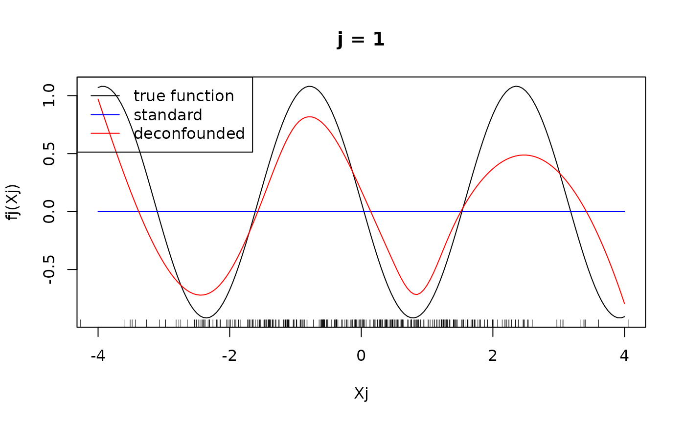

#> Warning in rug(X[, j]): some values will be clipped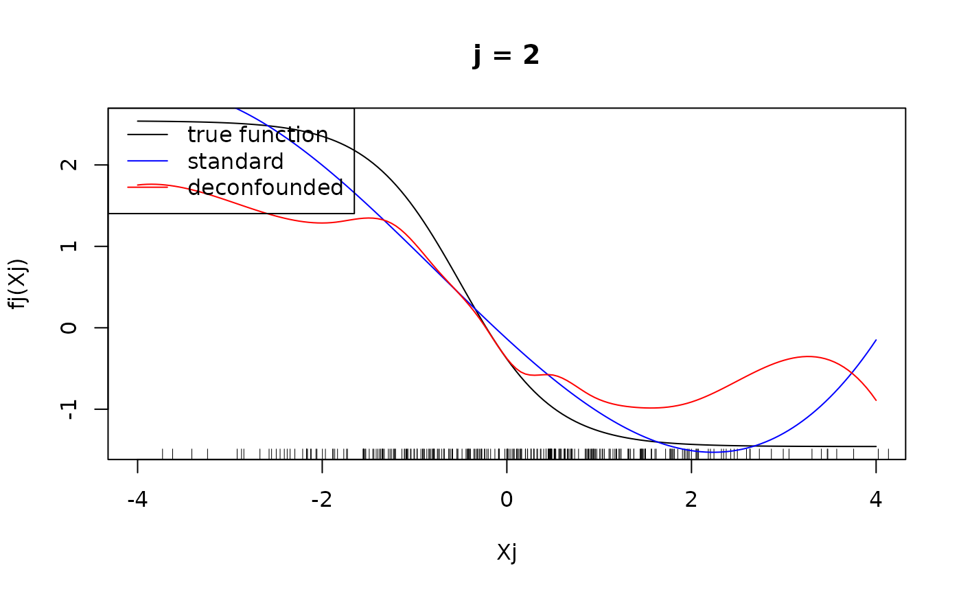

#> Warning in rug(X[, j]): some values will be clipped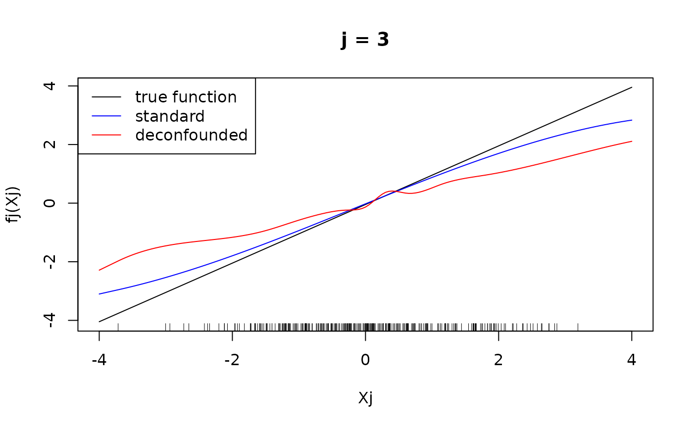

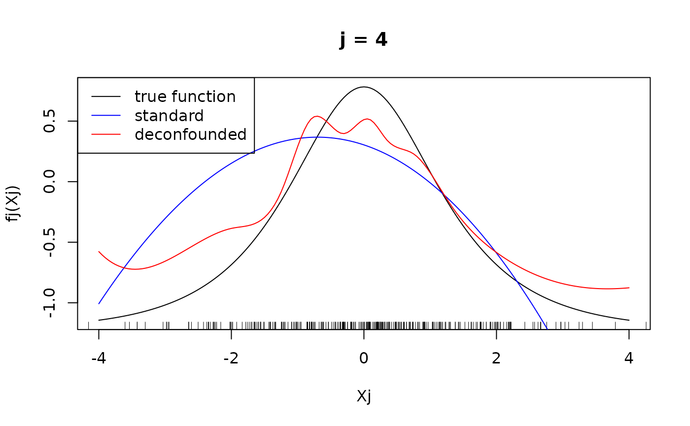
We see that for for $j = 2,3,4$, the difference in the fitted functions is not very large, at least in the regions, where there are many observations of $X_j$. However, the standard additive model failed to put $j=1$ into the active set and as seen above, attributed larger effects to the variables that are not in the true active set, hence leading to the significantly larger mean squared error observed above.

Scheidegger, Cyrill, Zijian Guo, and Peter Bühlmann. 2025. “Spectral Deconfounding for High-Dimensional Sparse Additive Models.” ACM / IMS J. Data Sci. https://doi.org/10.1145/3711116.