SDTree

In the following, we compare the Spectrally Deconfounded Regression Tree $f^{SDTree}(X)$ to the classical regression tree $f^{Tree}(X)$(Breiman et al. 2017) using simulated data from a confounded process. We simulate the data similar to simulate_data_nonlinear() but with a random regression tree, i.e. step-function for the direct relationship $f(X)$.

library(SDModels)

set.seed(99)

# number of confounding covariates in H
q <- 6

# number of covariates in X
p <- 500

# number of observations
n <- 500

# number of non-zero coefficients in beta
m <- 5
dat <- simulate_data_step(q, p, n, m, make_tree = TRUE)

Given the data, we can estimate both the SDTree and the classical regression tree. Here we estimate both trees with the default parameters. One could choose, for example, the regularization parameter cp in a more principled way than just setting it to 0.01, e.g. cvSDTree() or regPath.SDTree(). But 0.01 seem like a good first try and is also the default value in rpart (Therneau and Atkinson 2022).

dec_tree <- SDTree(x = dat$X, y = dat$Y, cp = 0.01)
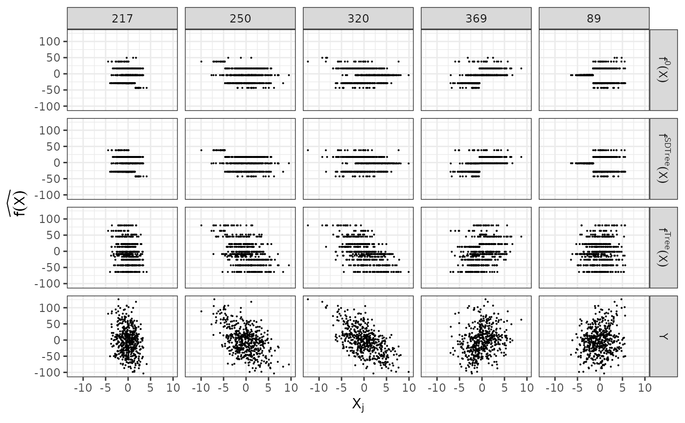
plain_tree <- SDTree(x = dat$X, y = dat$Y, Q_type = 'no_deconfounding', cp = 0.01)

Let us observe, what the different trees predict, by comparing the predictions to the true function and the observed response. On top, we show the underlying true step function $f^0(X)$ against the 5 covariates used for splitting partitions. On the bottom, we see the observed response $Y$. The SDTree $f^{SDTree}(X)$ predicts almost the same response as the true underlying function. The plain classical regression tree, on the other hand, results in a prediction close to the observed $\mathbf{Y}$.

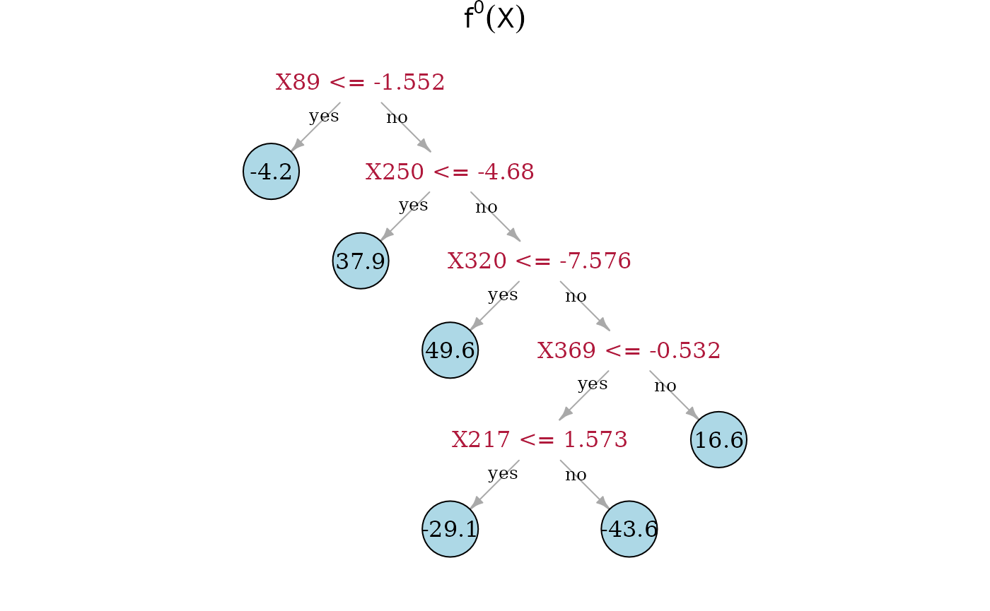
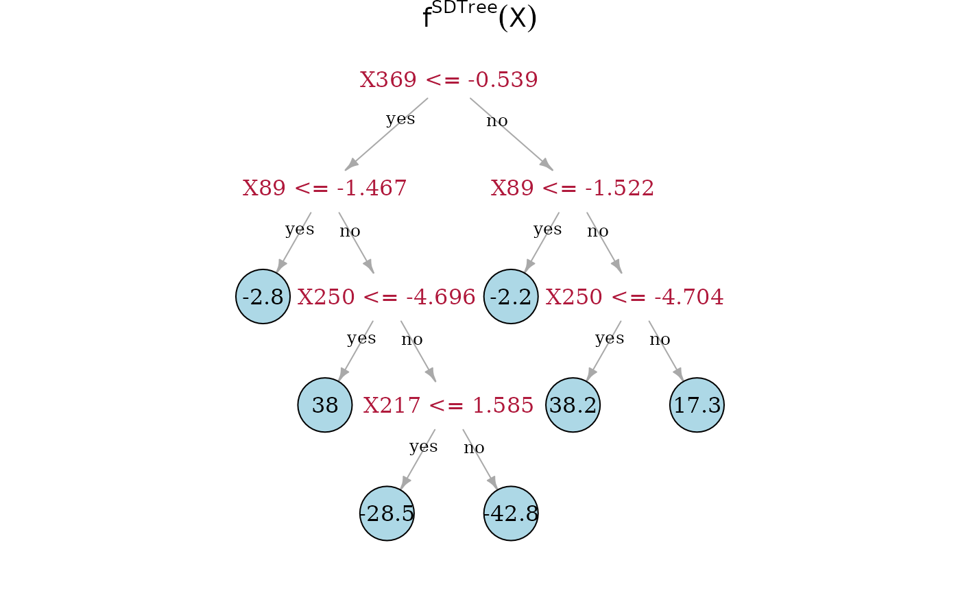
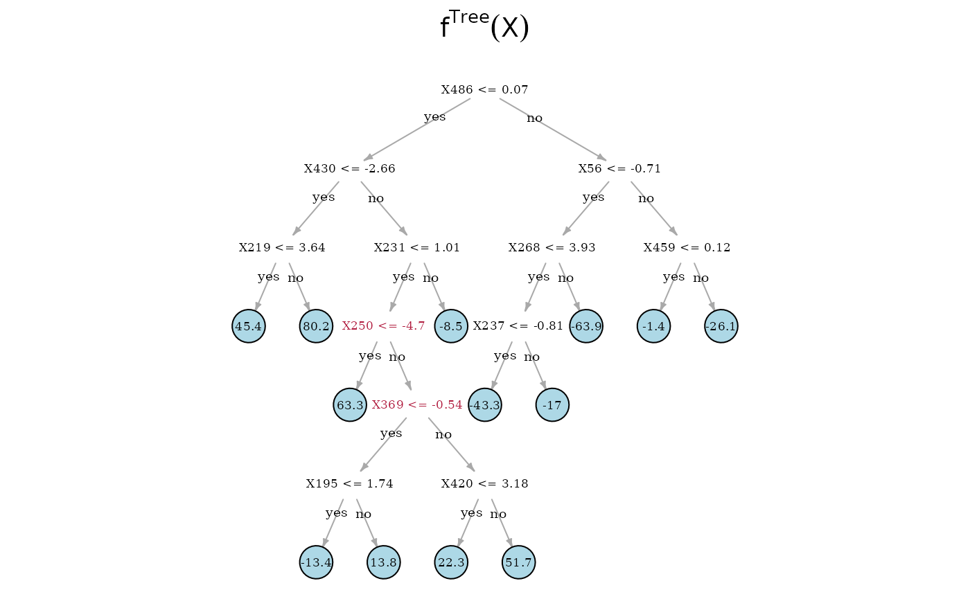
Now, we can directly look at the estimated tree structures. On top is the true underlying random regression tree, and below are the two tree estimates. In the middle is the SDTree and on the bottom is the plain classical regression tree. The nodes that choose a covariate for a split, that is also used in the true underlying causal function, are marked in red. Besides $X_{320}$, the SDTree uses all the parents of $Y$ for splits. Since $X_{320}$ only splits three observations into the node with a response level of 49.6, it seems reasonable that the noise and confounding in the observed data overshadow this effect. The order of the splits in the SDTree is partially different from the true function. $X_{369}$ is used too early resulting in having to split with $X_{250}$ and $X_{89}$ in both following subtrees. Estimating the partitions using no deconfounding results in the regression tree on the bottom. Here, we only find two of the parents of $Y$. Especially problematic is that the not deconfounded regression tree first splits with a few irrelevant covariates. Therefore, if an observation has $X_{486} > 0.07$ or $X_{430} \leq -2.66$, which has no meaning in the underlying function, no relevant split is left in the sub-tree.

Breiman, Leo, Jerome H. Friedman, Richard A. Olshen, and Charles J. Stone. 2017. Classification And Regression Trees. Routledge. https://doi.org/10.1201/9781315139470.

Therneau, Terry, and Beth Atkinson. 2022. “rpart: Recursive Partitioning and Regression Trees.” https://CRAN.R-project.org/package=rpart.